<?xml version="1.0" encoding="utf-8"?>
<feed xmlns="http://www.w3.org/2005/Atom">
  <author>
    <name>Bo Li</name>
  </author>
  <generator uri="https://hexo.io/">Hexo</generator>
  <id>https://bobboli.github.io/</id>
  <link href="https://bobboli.github.io/" rel="alternate"/>
  <link href="https://bobboli.github.io/atom.xml" rel="self"/>
  <rights>All rights reserved 2026, Bo Li</rights>
  <subtitle>Engineering notes on AI infrastructure, GPU computing, and systems</subtitle>
  <title>Bo Li</title>
  <updated>2026-07-12T17:44:15.212Z</updated>
  <entry>
    <author>
      <name>Bo Li</name>
    </author>
    <category term="Tech Blogs" scheme="https://bobboli.github.io/categories/Tech-Blogs/"/>
    <category term="TensorRT-LLM" scheme="https://bobboli.github.io/tags/TensorRT-LLM/"/>
    <category term="sparse-attention" scheme="https://bobboli.github.io/tags/sparse-attention/"/>
    <category term="LLM-inference" scheme="https://bobboli.github.io/tags/LLM-inference/"/>
    <category term="BLASST" scheme="https://bobboli.github.io/tags/BLASST/"/>
    <content>
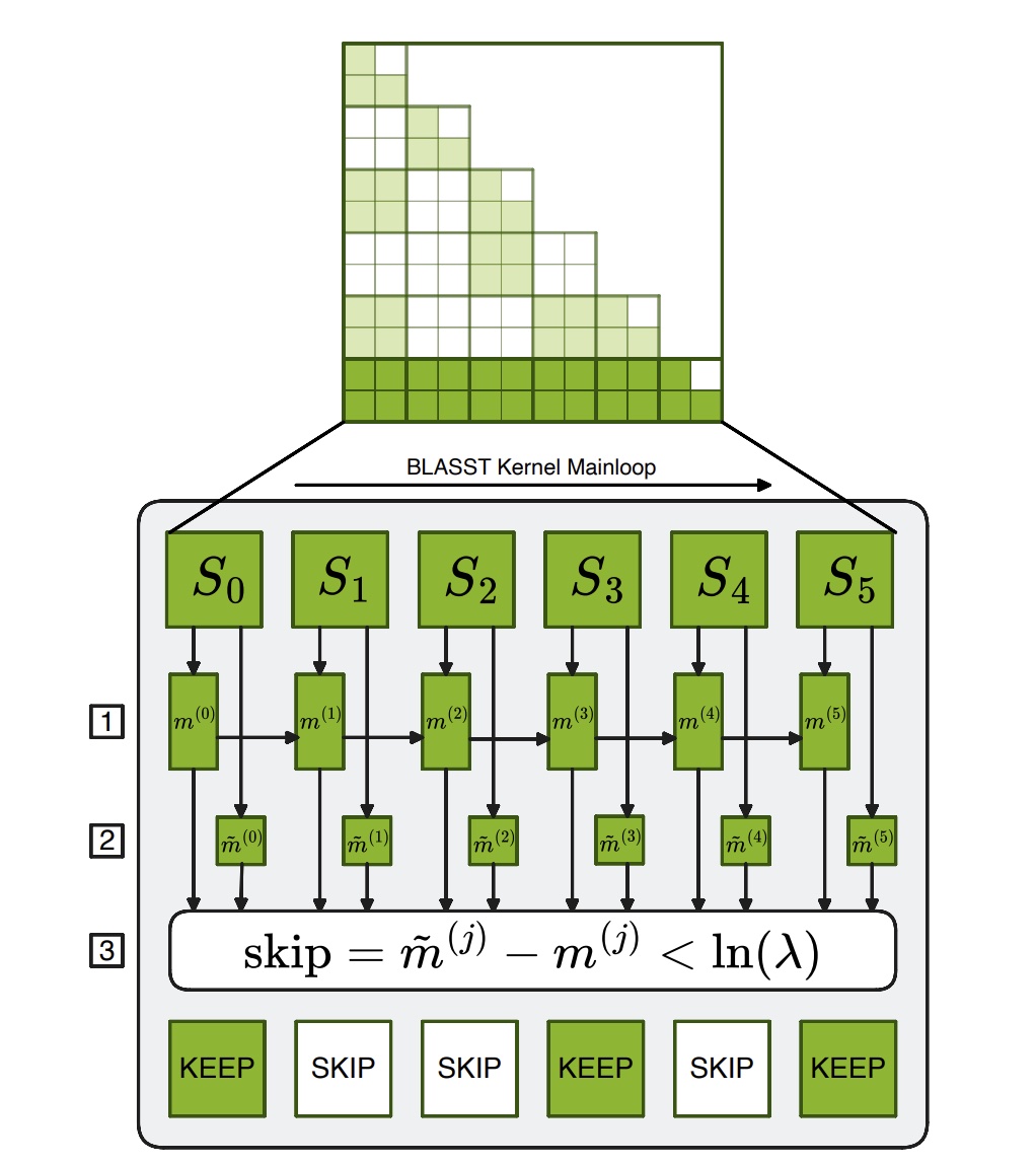
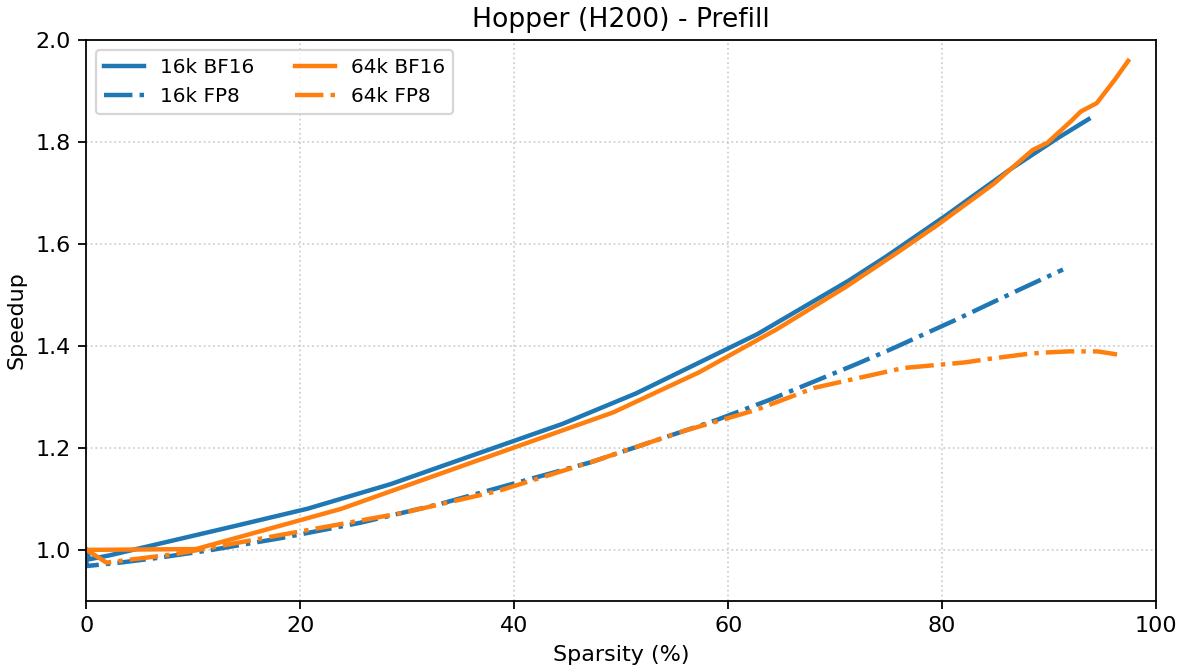
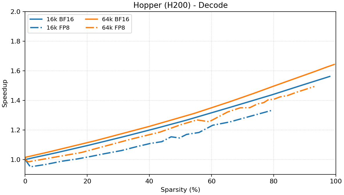
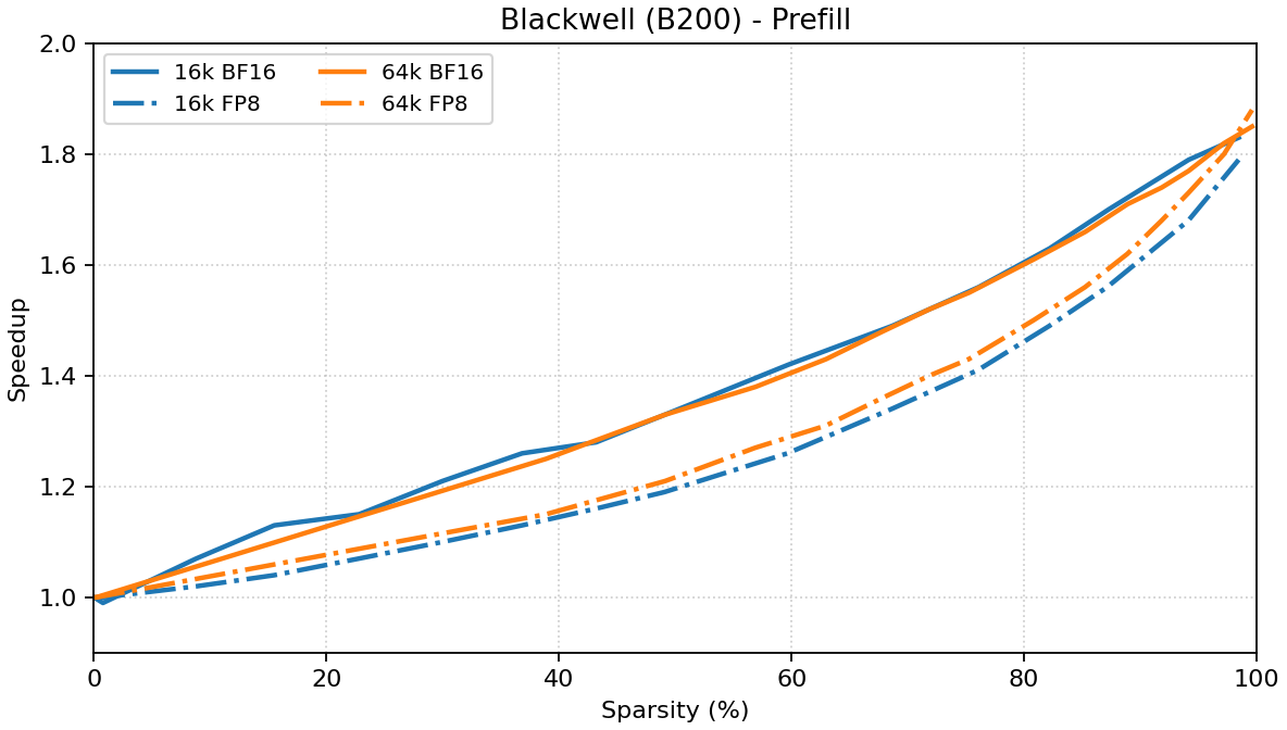
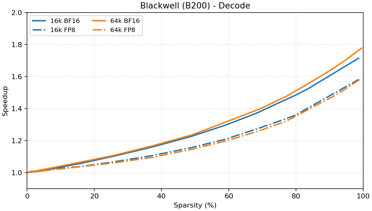
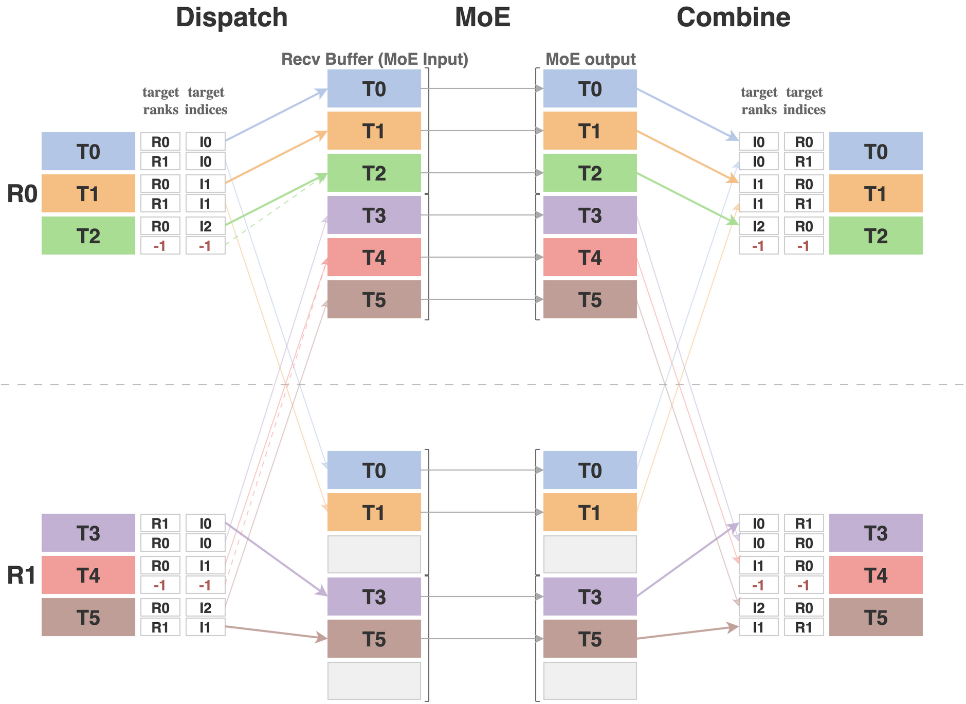
      <![CDATA[<blockquote><p><a href="https://nvidia.github.io/TensorRT-LLM/blogs/tech_blog/blog16_Accelerating_Long_Context_Inference_with_Skip_Softmax_Attention.html">Skip Softmax Attention</a> is a drop-in post-training sparse attention method and the productized implementation of <a href="https://arxiv.org/abs/2512.12087">BLASST</a> in NVIDIA TensorRT-LLM. It is available for accelerating both <a href="https://github.com/NVIDIA/TensorRT-LLM/blob/main/docs/source/features/sparse-attention.md#skip-softmax-attention">LLM workloads</a> and <a href="https://github.com/NVIDIA/TensorRT-LLM/blob/main/docs/source/visual-gen/features/sparse-attention.md#skip-softmax-attention">visual-generation workloads</a>.</p><p>The original article was published in <a href="https://github.com/NVIDIA/TensorRT-LLM/blob/main/docs/source/blogs/tech_blog/blog16_Accelerating_Long_Context_Inference_with_Skip_Softmax_Attention.md">NVIDIA TensorRT-LLM</a> and is embedded here for convenience.</p></blockquote><span id="more"></span><p>As context lengths grow from thousands to hundreds of thousands of tokens, attention computation becomes a major bottleneck in long-context LLM inference. TensorRT-LLM provides a <a href="https://nvidia.github.io/TensorRT-LLM/features/sparse-attention.html#framework-level-sparse-attention">sparse attention framework</a> that supports techniques like KV cache compression and sparse pattern prediction, featured in <a href="https://arxiv.org/pdf/2502.14051">RocketKV</a> and <a href="https://github.com/deepseek-ai/DeepSeek-V3.2-Exp/blob/main/DeepSeek_V3_2.pdf">DSA</a>. However, these require framework-level support—additional token selection steps, auxiliary data structures, and kernel modifications are required, compared to the vanilla attention architecture. This complexity introduces <strong>runtime overhead</strong> that can offset performance gains, particularly when context lengths are not long enough to amortize the extra work.</p><p>In this blog, we introduce <strong>Skip Softmax Attention</strong>, a drop-in sparse attention technique that is designed to accelerate the existing pretrained models that use standard attention mechanisms like MHA, GQA, or MLA. Skip Softmax Attention is built on top of the Flash Attention algorithm and only requires modifying the existing <strong>attention kernels</strong>. Due to this simplicity, the end-to-end performance gain is more predictable. In addition, it is only an approximation method of the attention kernel computation, making it compatible with nearly all the other features, such as FP8 attention, KV cache reuse, chunked prefill etc.</p><h2 id="Method-Overview"><a href="#Method-Overview" class="headerlink" title="Method Overview"></a>Method Overview</h2><p>The idea of Skip Softmax Attention is to compare the local maximum $\tilde{m}_i^{(j)}$ of $Q \cdot K^T$ with the running global maximum $m_i^{(j)}$, and skip the softmax (exp) and BMM2 calculation for blocks that are below a certain threshold $\lambda$:</p><div class="math-display">\[\exp(\tilde{m}_i^{(j)} - m_i^{(j)}) &lt; \lambda\]</div><p>In this way, we can indirectly control the sparsity via the threshold. The threshold is set to be inversely proportional to the context length, i.e., the longer the context, the smaller the threshold is needed to achieve the same sparsity.</p><p>The method is fully dynamic, and can be applied to both the prefilling and decoding. The algorithm of Skip Softmax Attention is described in the paper <a href="https://arxiv.org/pdf/2512.12087">BLASST: Dynamic Blocked Attention Sparsity via Softmax Thresholding</a>. We have also published a <a href="https://developer.nvidia.com/blog/accelerating-long-context-inference-with-skip-softmax-in-nvidia-tensorrt-llm/">Developer Blog</a> for explanation. Please refer to these resources for in-depth dive into the algorithm details. We will focus on the application of Skip Softmax Attention in TensorRT-LLM to accelerate long-context inference.</p><p align="center">  <img src="https://raw.githubusercontent.com/NVIDIA/TensorRT-LLM/1a349cd7a37e25ea6b69a98d355a64419d101b25/docs/source/blogs/media/tech_blog16_blasst.jpg" alt="BLASST Illustration" style="width: 50%; min-width: 300px; display: block; margin: auto;" /></p><h2 id="Example-Usage"><a href="#Example-Usage" class="headerlink" title="Example Usage"></a>Example Usage</h2><p>Enabling Skip Softmax Attention is pretty simple: we only need to configure the <code>SkipSoftmaxAttentionConfig</code> and pass it to the <code>LLM</code> API:</p><figure class="highlight python"><table><tr><td class="gutter"><pre><span class="line">1</span><br><span class="line">2</span><br><span class="line">3</span><br><span class="line">4</span><br><span class="line">5</span><br><span class="line">6</span><br><span class="line">7</span><br><span class="line">8</span><br><span class="line">9</span><br><span class="line">10</span><br><span class="line">11</span><br><span class="line">12</span><br><span class="line">13</span><br></pre></td><td class="code"><pre><span class="line"><span class="keyword">from</span> tensorrt_llm <span class="keyword">import</span> LLM</span><br><span class="line"><span class="keyword">from</span> tensorrt_llm.llmapi <span class="keyword">import</span> SkipSoftmaxAttentionConfig</span><br><span class="line"></span><br><span class="line">sparse_attention_config = SkipSoftmaxAttentionConfig(threshold_scale_factor=<span class="number">1000.0</span>)</span><br><span class="line"></span><br><span class="line"><span class="comment"># Additionally, the threshold_scale_factor for prefill and decode could be separately configured.</span></span><br><span class="line">sparse_attention_config = SkipSoftmaxAttentionConfig(threshold_scale_factor=&#123;<span class="string">&quot;prefill&quot;</span>: <span class="number">1000.0</span>, <span class="string">&quot;decode&quot;</span>: <span class="number">500.0</span>&#125;)</span><br><span class="line"></span><br><span class="line">llm = LLM(</span><br><span class="line">   model=<span class="string">&quot;Qwen/Qwen3-30B-A3B-Instruct-2507&quot;</span>,</span><br><span class="line">   sparse_attention_config=sparse_attention_config,</span><br><span class="line">   <span class="comment"># Other LLM arguments...</span></span><br><span class="line">)</span><br></pre></td></tr></table></figure><p>The configuration could also be specified through the extra LLM API options YAML file. An example to launch an OpenAI-compatible endpoint is shown below:</p><figure class="highlight bash"><table><tr><td class="gutter"><pre><span class="line">1</span><br><span class="line">2</span><br><span class="line">3</span><br><span class="line">4</span><br><span class="line">5</span><br><span class="line">6</span><br><span class="line">7</span><br><span class="line">8</span><br><span class="line">9</span><br><span class="line">10</span><br><span class="line">11</span><br><span class="line">12</span><br><span class="line">13</span><br><span class="line">14</span><br><span class="line">15</span><br><span class="line">16</span><br></pre></td><td class="code"><pre><span class="line"><span class="built_in">cat</span> &gt;extra_llm_api_options.yaml &lt;&lt;<span class="string">EOF</span></span><br><span class="line"><span class="string">sparse_attention_config:</span></span><br><span class="line"><span class="string">    algorithm: skip_softmax</span></span><br><span class="line"><span class="string">    threshold_scale_factor: 1000.0</span></span><br><span class="line"><span class="string">EOF</span></span><br><span class="line"></span><br><span class="line"><span class="comment"># Additionally, the threshold_scale_factor for prefill and decode could be separately configured.</span></span><br><span class="line"><span class="built_in">cat</span> &gt;extra_llm_api_options.yaml &lt;&lt;<span class="string">EOF</span></span><br><span class="line"><span class="string">sparse_attention_config:</span></span><br><span class="line"><span class="string">    algorithm: skip_softmax</span></span><br><span class="line"><span class="string">    threshold_scale_factor:</span></span><br><span class="line"><span class="string">        prefill: 1000.0</span></span><br><span class="line"><span class="string">        decode: 500.0</span></span><br><span class="line"><span class="string">EOF</span></span><br><span class="line"></span><br><span class="line">trtllm-serve Qwen/Qwen3-30B-A3B-Instruct-2507 --extra_llm_api_options extra_llm_api_options.yaml</span><br></pre></td></tr></table></figure><p>The actual threshold value equals the <code>threshold_scale_factor</code> divided by the context length. <a href="https://github.com/NVIDIA/Model-Optimizer">NVIDIA Model Optimizer</a> will support the calibration to automatically determine the required value given the target sparsity. We will use <code>Qwen3-30B-A3B-Instruct-2507</code> as the example model for testing, and the calibrated threshold scale factors are listed below:</p><table><thead><tr><th align="center">Target Sparsity</th><th align="center">Threshold Scale Factor (Prefill)</th><th align="center">Threshold Scale Factor (Decode)</th></tr></thead><tbody><tr><td align="center">0.0</td><td align="center">0.0</td><td align="center">0.0</td></tr><tr><td align="center">0.1</td><td align="center">18.76</td><td align="center">0.32</td></tr><tr><td align="center">0.2</td><td align="center">44.37</td><td align="center">0.86</td></tr><tr><td align="center">0.3</td><td align="center">104.97</td><td align="center">2.30</td></tr><tr><td align="center">0.4</td><td align="center">248.40</td><td align="center">6.17</td></tr><tr><td align="center">0.5</td><td align="center">587.18</td><td align="center">16.52</td></tr><tr><td align="center">0.6</td><td align="center">1390.63</td><td align="center">44.26</td></tr><tr><td align="center">0.7</td><td align="center">3293.04</td><td align="center">118.62</td></tr><tr><td align="center">0.8</td><td align="center">7799.91</td><td align="center">317.99</td></tr><tr><td align="center">0.9</td><td align="center">18471.56</td><td align="center">852.20</td></tr></tbody></table><h2 id="Accuracy-Evaluation"><a href="#Accuracy-Evaluation" class="headerlink" title="Accuracy Evaluation"></a>Accuracy Evaluation</h2><p>We evaluate the accuracy of Skip Softmax Attention using LongBench V1 and V2. LongBench V1 is a comprehensive benchmark for medium-to-long context understanding, with average sequence length of 10k tokens. LongBench V2 is a harder benchmark that contains longer sequences, and we pick its <code>medium</code> subset and truncate the prompt length to 256k due to the limit of the native context window of the model. The average sequence length of LongBench V2 is 130k tokens.</p><p>The evaluation results (on H200) are summarized in the table below:</p><table><thead><tr><th align="center">Target Sparsity</th><th align="center">LongBench V1 Overall Accuracy</th><th align="center">LongBench V2 Overall Accuracy</th></tr></thead><tbody><tr><td align="center">0.0</td><td align="center">47.79</td><td align="center">35.81</td></tr><tr><td align="center">0.1</td><td align="center">47.92</td><td align="center">40.00</td></tr><tr><td align="center">0.2</td><td align="center">47.80</td><td align="center">38.14</td></tr><tr><td align="center">0.3</td><td align="center">47.84</td><td align="center">38.60</td></tr><tr><td align="center">0.4</td><td align="center">47.84</td><td align="center">39.53</td></tr><tr><td align="center">0.5</td><td align="center">46.87</td><td align="center">37.67</td></tr><tr><td align="center">0.6</td><td align="center">46.45</td><td align="center">36.28</td></tr><tr><td align="center">0.7</td><td align="center">45.56</td><td align="center">34.88</td></tr><tr><td align="center">0.8</td><td align="center">43.38</td><td align="center">36.74</td></tr><tr><td align="center">0.9</td><td align="center">39.84</td><td align="center">39.07</td></tr></tbody></table><p>Note that the number of samples in LongBench V2 is very small (<del>200), so the result is subject to large variance. You will see non-monotonic relationship between sparsity and accuracy. We recommend to look at LongBench V1 (</del>5000 samples) for inspecting the accuracy loss trend.</p><h2 id="Performance-Benchmark"><a href="#Performance-Benchmark" class="headerlink" title="Performance Benchmark"></a>Performance Benchmark</h2><p>Skip Softmax Attention is supported on both Hopper and Blackwell GPUs and builds on top of the SoTA performance of the TensorRT-LLM’s attention kernels. Hopper prefilling is implemented in <a href="https://github.com/NVIDIA/TensorRT-LLM/tree/main/cpp/kernels/fmha_v2">fmha_v2</a>, Hopper decoding is implemented in <a href="https://github.com/NVIDIA/TensorRT-LLM/tree/main/cpp/kernels/xqa">XQA</a>, and Blackwell is implemented in <a href="https://github.com/NVIDIA/TensorRT-LLM/tree/main/cpp/tensorrt_llm/kernels/trtllmGenKernels">trtllm-gen</a>.</p><h3 id="Kernel-Performance"><a href="#Kernel-Performance" class="headerlink" title="Kernel Performance"></a>Kernel Performance</h3><p>We provide the performance data of the attention kernels under different achieved sparsity by specifying the threshold. The micro-benchmarking is performed under these configs: q_heads&#x3D;64, kv_heads&#x3D;4, head_dim&#x3D;128, seqlen&#x3D;16k&#x2F;64k. Both BF16 and FP8 attention are supported. For prefilling, batch size is set to 1; for decoding, batch size is 64.</p><p>As a reference, the baseline performance data <strong>without</strong> Skip Softmax Attention are listed below (you can fill in the numbers).</p><p><strong>Prefill Baseline (we report compute performance in TFLOP&#x2F;s):</strong></p><table><thead><tr><th align="center">GPU</th><th align="center">Seqlen</th><th align="center">Precision</th><th align="right">TFLOP&#x2F;s</th><th align="right">Duration µs</th></tr></thead><tbody><tr><td align="center">H200</td><td align="center">16k</td><td align="center">BF16</td><td align="right">594.05</td><td align="right">7403</td></tr><tr><td align="center">H200</td><td align="center">16k</td><td align="center">FP8</td><td align="right">852.81</td><td align="right">5157</td></tr><tr><td align="center">H200</td><td align="center">64k</td><td align="center">BF16</td><td align="right">610.30</td><td align="right">115301</td></tr><tr><td align="center">H200</td><td align="center">64k</td><td align="center">FP8</td><td align="right">873.60</td><td align="right">80550</td></tr><tr><td align="center">B200</td><td align="center">16k</td><td align="center">BF16</td><td align="right">1029.13</td><td align="right">4273</td></tr><tr><td align="center">B200</td><td align="center">16k</td><td align="center">FP8</td><td align="right">1523.57</td><td align="right">2886</td></tr><tr><td align="center">B200</td><td align="center">64k</td><td align="center">BF16</td><td align="right">1038.26</td><td align="right">67775</td></tr><tr><td align="center">B200</td><td align="center">64k</td><td align="center">FP8</td><td align="right">1621.41</td><td align="right">43399</td></tr></tbody></table><p><strong>Decode Baseline (we report memory bandwidth in TB&#x2F;s):</strong></p><table><thead><tr><th align="center">GPU</th><th align="center">Seqlen</th><th align="center">Precision</th><th align="right">TB&#x2F;s</th><th align="right">Duration µs</th></tr></thead><tbody><tr><td align="center">H200</td><td align="center">16k</td><td align="center">BF16</td><td align="right">4.31</td><td align="right">498</td></tr><tr><td align="center">H200</td><td align="center">16k</td><td align="center">FP8</td><td align="right">4.03</td><td align="right">266</td></tr><tr><td align="center">H200</td><td align="center">64k</td><td align="center">BF16</td><td align="right">4.37</td><td align="right">1962</td></tr><tr><td align="center">H200</td><td align="center">64k</td><td align="center">FP8</td><td align="right">4.10</td><td align="right">1045</td></tr><tr><td align="center">B200</td><td align="center">16k</td><td align="center">BF16</td><td align="right">7.08</td><td align="right">303</td></tr><tr><td align="center">B200</td><td align="center">16k</td><td align="center">FP8</td><td align="right">5.46</td><td align="right">196</td></tr><tr><td align="center">B200</td><td align="center">64k</td><td align="center">BF16</td><td align="right">7.10</td><td align="right">1209</td></tr><tr><td align="center">B200</td><td align="center">64k</td><td align="center">FP8</td><td align="right">5.68</td><td align="right">755</td></tr></tbody></table><p>The following figures plot <strong>speedup vs. achieved sparsity</strong>, on top of the baseline performance:</p><table style="width: 100%; border: 0;">  <tr>    <td style="width: 50%; padding: 0 8px; vertical-align: top;">      <p align="center"><b>Hopper (H200)</b></p>      <p align="center"><b>Prefill</b></p>      <img src="https://raw.githubusercontent.com/NVIDIA/TensorRT-LLM/1a349cd7a37e25ea6b69a98d355a64419d101b25/docs/source/blogs/media/tech_blog16_hopper_prefill.png" alt="Hopper prefill kernel" style="width: 100%; min-width: 280px; display: block; margin: auto;" />      <p align="center"><b>Decode</b></p>      <img src="https://raw.githubusercontent.com/NVIDIA/TensorRT-LLM/1a349cd7a37e25ea6b69a98d355a64419d101b25/docs/source/blogs/media/tech_blog16_hopper_decode.png" alt="Hopper decode kernel" style="width: 100%; min-width: 280px; display: block; margin: auto;" />    </td>    <td style="width: 50%; padding: 0 8px; vertical-align: top;">      <p align="center"><b>Blackwell (B200)</b></p>      <p align="center"><b>Prefill</b></p>      <img src="https://raw.githubusercontent.com/NVIDIA/TensorRT-LLM/1a349cd7a37e25ea6b69a98d355a64419d101b25/docs/source/blogs/media/tech_blog16_blackwell_prefill.png" alt="Blackwell prefill kernel" style="width: 100%; min-width: 280px; display: block; margin: auto;" />      <p align="center"><b>Decode</b></p>      <img src="https://raw.githubusercontent.com/NVIDIA/TensorRT-LLM/1a349cd7a37e25ea6b69a98d355a64419d101b25/docs/source/blogs/media/tech_blog16_blackwell_decode.png" alt="Blackwell decode kernel" style="width: 100%; min-width: 280px; display: block; margin: auto;" />    </td>  </tr></table><p>Skip Softmax Attention could further boost the performance of FP8 attention, though the gain is less significant compared to BF16.</p><h3 id="End-to-end-Performance"><a href="#End-to-end-Performance" class="headerlink" title="End-to-end Performance"></a>End-to-end Performance</h3><p>We benchmark the end-to-end performance to demonstrate the benefit of Skip Softmax Attention. Due to the quadratic complexity of the attention, the TTFT in long-context scenarios is often a severe blocker for real-world usage. Skip Softmax Attention can significantly reduce the TTFT by accelerating the prefilling kernel, and the TPOT can also be reduced if the context length is long enough. The experiment is conducted on a single H200 or B200 GPU, using the exact same dataset as the accuracy evaluation.</p><p><strong>LongBench V1, avg ISL&#x3D;10k, OSL&#x3D;6:</strong></p><table><thead><tr><th align="center">Target Sparsity</th><th align="right">TTFT&#x2F;ms (H200)</th><th align="right">TPOT&#x2F;ms (H200)</th><th align="right">TTFT&#x2F;ms (B200)</th><th align="right">TPOT&#x2F;ms (B200)</th></tr></thead><tbody><tr><td align="center">0.0</td><td align="right">9419.61</td><td align="right">1731.80</td><td align="right">4854.55</td><td align="right">928.45</td></tr><tr><td align="center">0.1</td><td align="right">9519.40</td><td align="right">1746.73</td><td align="right">4758.06</td><td align="right">909.08</td></tr><tr><td align="center">0.2</td><td align="right">9417.36</td><td align="right">1729.74</td><td align="right">4794.23</td><td align="right">916.64</td></tr><tr><td align="center">0.3</td><td align="right">9304.48</td><td align="right">1711.27</td><td align="right">4770.26</td><td align="right">913.51</td></tr><tr><td align="center">0.4</td><td align="right">9139.85</td><td align="right">1684.78</td><td align="right">4672.09</td><td align="right">896.25</td></tr><tr><td align="center">0.5</td><td align="right">8847.43</td><td align="right">1633.08</td><td align="right">4548.07</td><td align="right">873.80</td></tr><tr><td align="center">0.6</td><td align="right">8437.45</td><td align="right">1560.64</td><td align="right">4459.08</td><td align="right">858.60</td></tr><tr><td align="center">0.7</td><td align="right">8134.72</td><td align="right">1508.60</td><td align="right">4385.12</td><td align="right">846.64</td></tr><tr><td align="center">0.8</td><td align="right">8107.73</td><td align="right">1507.82</td><td align="right">4348.80</td><td align="right">831.88</td></tr><tr><td align="center">0.9</td><td align="right">8130.39</td><td align="right">1516.16</td><td align="right">4150.44</td><td align="right">798.93</td></tr></tbody></table><p>LongBench V1 results are reported with concurrency 64. Due to the nature of in-flight batching, the decoding requests might be piggybacked with the prefilling requests, so the TPOT is relatively high.</p><p><strong>LongBench V2, avg ISL&#x3D;130k, OSL&#x3D;200:</strong></p><table><thead><tr><th align="center">Target Sparsity</th><th align="right">TTFT&#x2F;ms (H200)</th><th align="right">TPOT&#x2F;ms (H200)</th><th align="right">TTFT&#x2F;ms (B200)</th><th align="right">TPOT&#x2F;ms (B200)</th></tr></thead><tbody><tr><td align="center">0.0</td><td align="right">16486.70</td><td align="right">9.34</td><td align="right">6990.59</td><td align="right">6.30</td></tr><tr><td align="center">0.1</td><td align="right">16487.54</td><td align="right">8.61</td><td align="right">7024.50</td><td align="right">6.30</td></tr><tr><td align="center">0.2</td><td align="right">16169.69</td><td align="right">8.61</td><td align="right">6687.21</td><td align="right">6.34</td></tr><tr><td align="center">0.3</td><td align="right">15750.17</td><td align="right">8.46</td><td align="right">6616.12</td><td align="right">6.33</td></tr><tr><td align="center">0.4</td><td align="right">15288.68</td><td align="right">8.61</td><td align="right">6432.32</td><td align="right">6.27</td></tr><tr><td align="center">0.5</td><td align="right">14554.04</td><td align="right">8.45</td><td align="right">6193.92</td><td align="right">6.29</td></tr><tr><td align="center">0.6</td><td align="right">14323.08</td><td align="right">8.44</td><td align="right">5966.53</td><td align="right">6.32</td></tr><tr><td align="center">0.7</td><td align="right">13871.32</td><td align="right">8.42</td><td align="right">5769.19</td><td align="right">6.31</td></tr><tr><td align="center">0.8</td><td align="right">12922.99</td><td align="right">8.58</td><td align="right">5605.66</td><td align="right">6.23</td></tr><tr><td align="center">0.9</td><td align="right">12507.95</td><td align="right">8.58</td><td align="right">5276.67</td><td align="right">6.29</td></tr></tbody></table><p>Due to the extremely long context length, we only run LongBench V2 with concurrency 1. In this scenario, the prefilling&#x2F;decoding is better separated and we can observe how is TTFT&#x2F;TPOT affected by the sparsity. Note that the speedup for decoding is less pronounced under small batch size. Small batch size and small number of heads (with TP) are more close to real-world usage for long-context serving due to the limit of SLO, and we are actively optimizing the decoding performance under such scenarios.</p><h2 id="Reproduction"><a href="#Reproduction" class="headerlink" title="Reproduction"></a>Reproduction</h2><p>We provide the commands to reproduce the results in the previous context, as a showcase of how to evaluate the accuracy and benchmark the performance for Skip Softmax Attention.</p><h3 id="Accuracy-evaluation-LongBench-V1-V2"><a href="#Accuracy-evaluation-LongBench-V1-V2" class="headerlink" title="Accuracy evaluation (LongBench V1&#x2F;V2)"></a>Accuracy evaluation (LongBench V1&#x2F;V2)</h3><p>Both LongBench V1 and V2 are integrated into the TensorRT-LLM accuracy test suite, <code>trtllm-eval</code>. Here are the example scripts to run the accuracy evaluation:</p><figure class="highlight bash"><table><tr><td class="gutter"><pre><span class="line">1</span><br><span class="line">2</span><br><span class="line">3</span><br><span class="line">4</span><br><span class="line">5</span><br><span class="line">6</span><br><span class="line">7</span><br><span class="line">8</span><br><span class="line">9</span><br><span class="line">10</span><br></pre></td><td class="code"><pre><span class="line"><span class="comment"># Dump the extra LLM API options YAML file.</span></span><br><span class="line"><span class="built_in">cat</span> &gt;extra_llm_api_options.yaml &lt;&lt;<span class="string">EOF</span></span><br><span class="line"><span class="string">kv_cache_config:</span></span><br><span class="line"><span class="string">    free_gpu_memory_fraction: 0.8</span></span><br><span class="line"><span class="string">sparse_attention_config:</span></span><br><span class="line"><span class="string">    algorithm: skip_softmax</span></span><br><span class="line"><span class="string">    threshold_scale_factor:</span></span><br><span class="line"><span class="string">        prefill: $&#123;thr_prefill&#125;</span></span><br><span class="line"><span class="string">        decode: $&#123;thr_decode&#125;</span></span><br><span class="line"><span class="string">EOF</span></span><br></pre></td></tr></table></figure><figure class="highlight bash"><table><tr><td class="gutter"><pre><span class="line">1</span><br><span class="line">2</span><br><span class="line">3</span><br><span class="line">4</span><br><span class="line">5</span><br><span class="line">6</span><br></pre></td><td class="code"><pre><span class="line"><span class="comment"># Evaluate LongBench V1.</span></span><br><span class="line">trtllm-eval --model Qwen/Qwen3-30B-A3B-Instruct-2507 \</span><br><span class="line"> --max_batch_size 64 --max_num_tokens 100000 \</span><br><span class="line"> --extra_llm_api_options extra_llm_api_options.yaml \</span><br><span class="line"> longbench_v1 \</span><br><span class="line"> --output_dir <span class="variable">$&#123;OUTPUT_DIR&#125;</span>  <span class="comment"># Dump dataset for perf benching</span></span><br></pre></td></tr></table></figure><figure class="highlight bash"><table><tr><td class="gutter"><pre><span class="line">1</span><br><span class="line">2</span><br><span class="line">3</span><br><span class="line">4</span><br><span class="line">5</span><br><span class="line">6</span><br><span class="line">7</span><br><span class="line">8</span><br></pre></td><td class="code"><pre><span class="line"><span class="comment"># Evaluate LongBench V2.</span></span><br><span class="line">trtllm-eval --model Qwen/Qwen3-30B-A3B-Instruct-2507 \</span><br><span class="line">--max_batch_size 1 --max_num_tokens 262144 \</span><br><span class="line">--extra_llm_api_options extra_llm_api_options.yaml \</span><br><span class="line">longbench_v2 \</span><br><span class="line">--length medium \  <span class="comment"># Medium subset of LongBench V2</span></span><br><span class="line">--max_input_length 256000 \  <span class="comment"># Truncate the prompt length to 256k</span></span><br><span class="line">--output_dir <span class="variable">$&#123;OUTPUT_DIR&#125;</span>  <span class="comment"># Dump dataset for perf benching</span></span><br></pre></td></tr></table></figure><h3 id="End-to-end-performance-TTFT-TPOT"><a href="#End-to-end-performance-TTFT-TPOT" class="headerlink" title="End-to-end performance (TTFT&#x2F;TPOT)"></a>End-to-end performance (TTFT&#x2F;TPOT)</h3><p>The option <code>--output_dir</code> in <code>trtllm-eval</code> will dump the dataset in the format required by <code>trtllm-bench</code> as <code>dumped_ids.json</code>. After getting the data, we can perform end-to-end benchmarking:</p><figure class="highlight bash"><table><tr><td class="gutter"><pre><span class="line">1</span><br><span class="line">2</span><br><span class="line">3</span><br><span class="line">4</span><br><span class="line">5</span><br><span class="line">6</span><br><span class="line">7</span><br></pre></td><td class="code"><pre><span class="line"><span class="comment"># Benchmark on LongBench V1.</span></span><br><span class="line">trtllm-bench --model Qwen/Qwen3-30B-A3B-Instruct-2507 \</span><br><span class="line">throughput --dataset <span class="variable">$&#123;OUTPUT_DIR&#125;</span>/dumped_ids.json \</span><br><span class="line">--concurrency 64 --max_batch_size 64 --max_num_tokens 100000 \</span><br><span class="line">--extra_llm_api_options extra_llm_api_options.yaml \</span><br><span class="line">--warmup 0 --streaming \</span><br><span class="line">--report_json <span class="variable">$&#123;OUTPUT_DIR&#125;</span>/report.json</span><br></pre></td></tr></table></figure><figure class="highlight bash"><table><tr><td class="gutter"><pre><span class="line">1</span><br><span class="line">2</span><br><span class="line">3</span><br><span class="line">4</span><br><span class="line">5</span><br><span class="line">6</span><br><span class="line">7</span><br></pre></td><td class="code"><pre><span class="line"><span class="comment"># Benchmark on LongBench V2.</span></span><br><span class="line">trtllm-bench --model Qwen/Qwen3-30B-A3B-Instruct-2507 \</span><br><span class="line">throughput --dataset <span class="variable">$&#123;OUTPUT_DIR&#125;</span>/dumped_ids.json \</span><br><span class="line">--concurrency 1 --max_batch_size 1 --max_num_tokens 262144 \</span><br><span class="line">--extra_llm_api_options extra_llm_api_options.yaml \</span><br><span class="line">--warmup 0 --streaming \</span><br><span class="line">--report_json <span class="variable">$&#123;OUTPUT_DIR&#125;</span>/report.json</span><br></pre></td></tr></table></figure><h2 id="Conclusion"><a href="#Conclusion" class="headerlink" title="Conclusion"></a>Conclusion</h2><p>Skip Softmax Attention is a kernel-based solution for accelerating the attention. Due to the design that BMM1 ($Q \cdot K^T$) in the attention kernel is not skipped, the performance gain is capped to 1.8x at kernel level. Nevertheless, it excels at achieving high sparsity with minimal accuracy degradation, and is especially effective in the medium-to-long context scenarios where previous methods like MInference cannot well handle, because the introduced runtime overhead may not pay off the speedup of the attention kernel. The drop-in nature of Skip Softmax Attention makes it a flexible, easy-to-use method for accelerating long-context inference. The Skip Softmax Attention kernels will also be <a href="https://github.com/flashinfer-ai/flashinfer/issues/2306">available in FlashInfer</a> for adoptions by the open-source community.</p>]]>
    </content>
    <id>https://bobboli.github.io/tech-blogs/accelerating-long-context-inference-with-skip-softmax-attention/</id>
    <link href="https://bobboli.github.io/tech-blogs/accelerating-long-context-inference-with-skip-softmax-attention/"/>
    <published>2026-07-12T16:02:00.000Z</published>
    <summary>
      <![CDATA[<blockquote>
<p><a href="https://nvidia.github.io/TensorRT-LLM/blogs/tech_blog/blog16_Accelerating_Long_Context_Inference_with_Skip_Softmax_Attention.html">Skip Softmax Attention</a> is a drop-in post-training sparse attention method and the productized implementation of <a href="https://arxiv.org/abs/2512.12087">BLASST</a> in NVIDIA TensorRT-LLM. It is available for accelerating both <a href="https://github.com/NVIDIA/TensorRT-LLM/blob/main/docs/source/features/sparse-attention.md#skip-softmax-attention">LLM workloads</a> and <a href="https://github.com/NVIDIA/TensorRT-LLM/blob/main/docs/source/visual-gen/features/sparse-attention.md#skip-softmax-attention">visual-generation workloads</a>.</p>
<p>The original article was published in <a href="https://github.com/NVIDIA/TensorRT-LLM/blob/main/docs/source/blogs/tech_blog/blog16_Accelerating_Long_Context_Inference_with_Skip_Softmax_Attention.md">NVIDIA TensorRT-LLM</a> and is embedded here for convenience.</p>
</blockquote>]]>
    </summary>
    <title>Accelerating Long-Context Inference with Skip Softmax Attention</title>
    <updated>2026-07-12T17:44:15.212Z</updated>
  </entry>
  <entry>
    <author>
      <name>Bo Li</name>
    </author>
    <category term="Tech Blogs" scheme="https://bobboli.github.io/categories/Tech-Blogs/"/>
    <category term="TensorRT-LLM" scheme="https://bobboli.github.io/tags/TensorRT-LLM/"/>
    <category term="MoE" scheme="https://bobboli.github.io/tags/MoE/"/>
    <category term="NVLink" scheme="https://bobboli.github.io/tags/NVLink/"/>
    <category term="GPU-communication" scheme="https://bobboli.github.io/tags/GPU-communication/"/>
    <content>
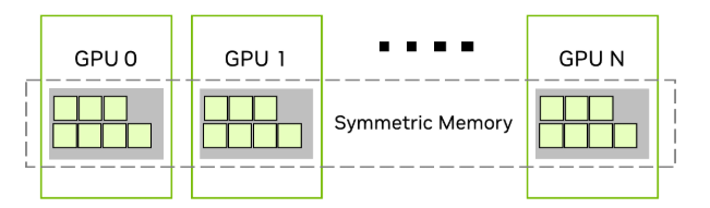
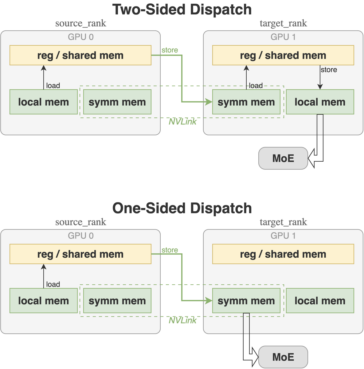
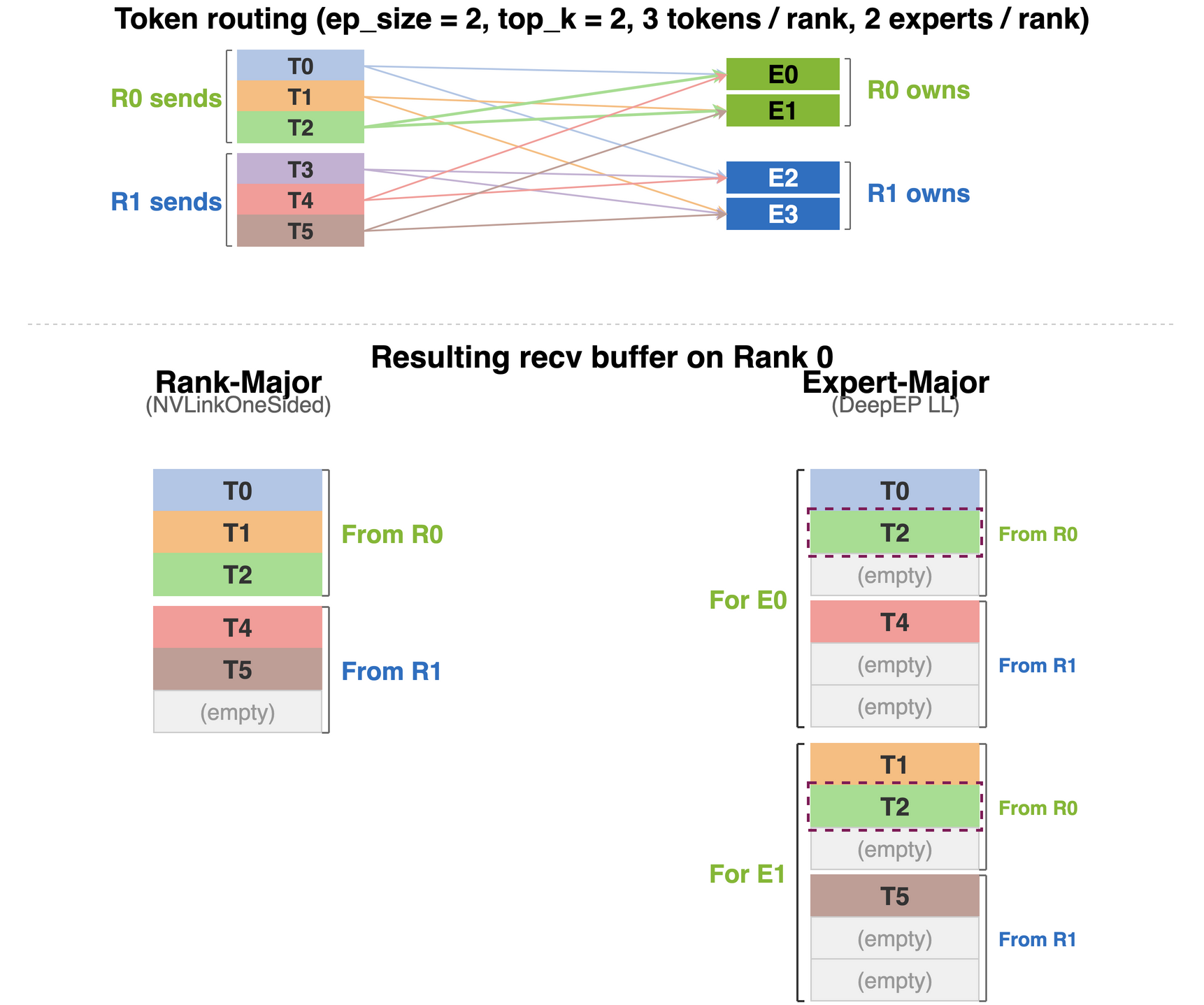
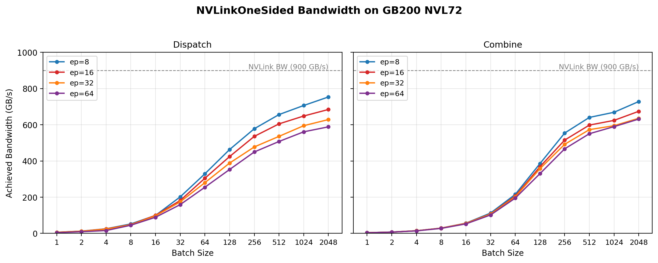
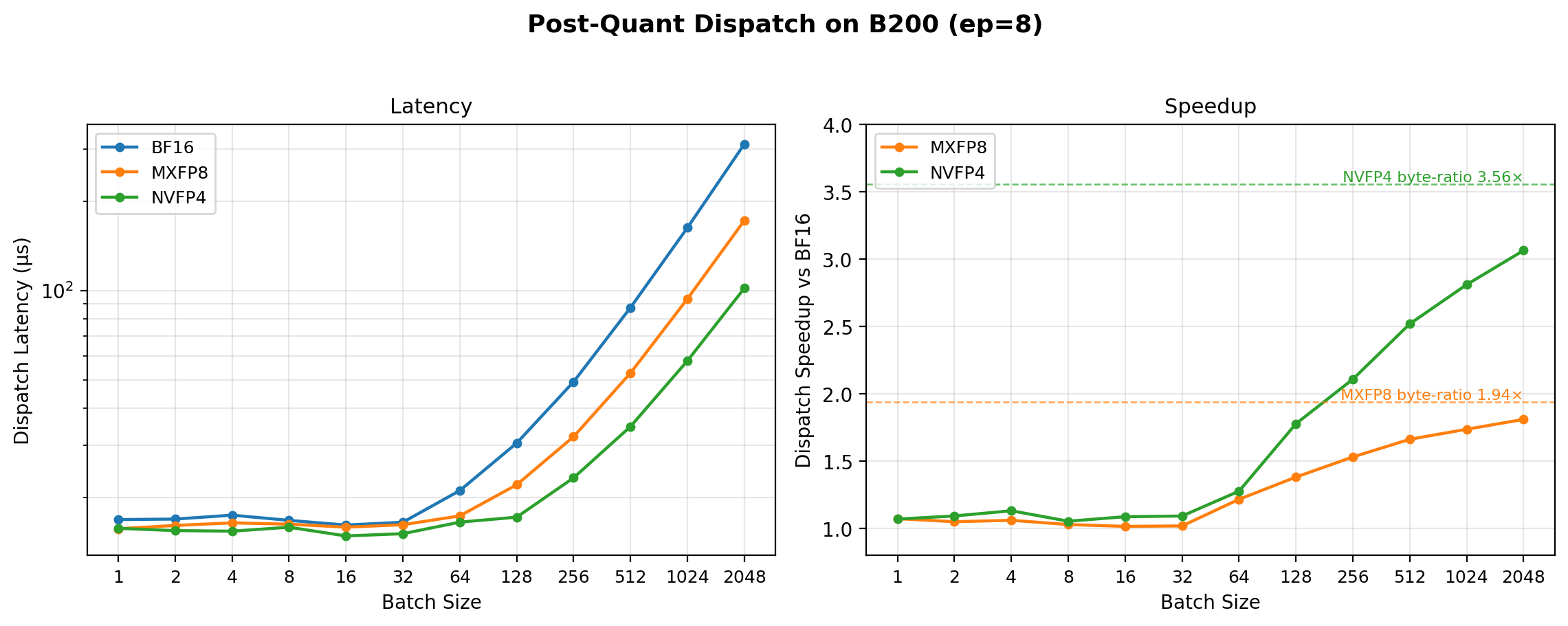
      <![CDATA[<blockquote><p><a href="https://nvidia.github.io/TensorRT-LLM/blogs/tech_blog/blog18_Optimizing_MoE_Communication_with_One_Sided_AlltoAll_Over_NVLink.html">This one-sided AlltoAll design</a> for MoE EP communication originated in <a href="https://github.com/NVIDIA/TensorRT-LLM/blob/main/docs/source/blogs/tech_blog/blog18_Optimizing_MoE_Communication_with_One_Sided_AlltoAll_Over_NVLink.md">NVIDIA TensorRT-LLM</a> and has since been ported to <a href="https://docs.flashinfer.ai/api/comm.html#flashinfer.comm.MoeAlltoAll">FlashInfer</a>. It is currently the fastest available MoE EP AlltoAll implementation for inference on NVLink and has been integrated into <a href="https://docs.vllm.ai/en/latest/serving/expert_parallel_deployment/#backend-selection-guide">vLLM</a> and <a href="https://sgl-project-sglang-93.mintlify.app/distributed/expert-parallelism#all-to-all-backends-moe-a2a-backend">SGLang</a>. A <a href="https://www.bilibili.com/video/BV1NQGx6mELa/">presentation</a> (in Chinese) is also available.</p><p>The original article was published in <a href="https://github.com/NVIDIA/TensorRT-LLM/blob/main/docs/source/blogs/tech_blog/blog18_Optimizing_MoE_Communication_with_One_Sided_AlltoAll_Over_NVLink.md">NVIDIA TensorRT-LLM</a> and is embedded here for convenience.</p></blockquote><span id="more"></span><p>Large-scale Mixture-of-Experts (MoE) models have become the dominant architecture for open-source LLMs. For inference, a common parallel strategy is <strong>Attention Data Parallel (DP) + MoE Expert Parallel (EP)</strong>: each GPU handles a portion of the requests (thus tokens) for attention and a portion of the experts for MoE. Since a token’s routed experts may reside on other GPUs, efficient communication is crucial for performance.</p><p>In this blog, we introduce <strong>NVLinkOneSided AlltoAll</strong>, the MoE communication kernels in TensorRT LLM designed for NVLink-connected systems (DGX B200, GB200 NVL72, etc.). We describe the key design choices, implementation details and performance benchmark results.</p><h2 id="Background"><a href="#Background" class="headerlink" title="Background"></a>Background</h2><p>There are two communication patterns that can be used between attention DP and MoE EP:</p><p><strong>1. AllGather + ReduceScatter.</strong> After attention, AllGather brings all tokens to every rank. Each rank computes MoE on the full token set using its local experts. After MoE, ReduceScatter sums the partial results back to each rank.</p><p><strong>2. AlltoAll (Dispatch + Combine).</strong> AllGather is redundant: if a token is not routed to any expert on a given rank, it does not need to be communicated there. The waste is especially significant when the EP size is larger than <code>top_k</code>, since a token is routed to at most <code>top_k</code> experts. AlltoAll sends each token only to the ranks that own its routed experts, eliminating the redundancy. The AlltoAll after attention is called <strong>dispatch</strong> and the AlltoAll after MoE is called <strong>combine</strong>.</p><p>Concretely, the total message size of AllGather&#x2F;ReduceScatter scales as <code>ep_size × num_tokens_per_rank × hidden_dim</code> (including data movement to self), while AlltoAll scales as <code>top_k × num_tokens_per_rank × hidden_dim</code>, since each token is dispatched to at most <code>top_k</code> target ranks. When <code>ep_size &gt; top_k</code>, AlltoAll communicates strictly less data.</p><h2 id="Design-Overview"><a href="#Design-Overview" class="headerlink" title="Design Overview"></a>Design Overview</h2><p>NVLinkOneSided AlltoAll rests on three design ideas:</p><ul><li><strong>One-sided data movement</strong> — each kernel only reads OR only writes peer memory, eliminating cooperative send&#x2F;recv and the extra copies it implies.</li><li><strong>Rank-major recv buffer</strong> — slots are indexed by source rank with no <code>top_k</code> duplication, shrinking buffer size and saving redundant communication.</li><li><strong>Flexible interface</strong> — quantization-agnostic data path, with a small API that exposes the recv buffer directly to the MoE module.</li></ul><p>The remainder of this section walks through the NVLink symmetric memory substrate that the kernels are built on, then each of the three ideas in turn.</p><h3 id="NVLink-Symmetric-Memory"><a href="#NVLink-Symmetric-Memory" class="headerlink" title="NVLink Symmetric Memory"></a>NVLink Symmetric Memory</h3><p>Communication across GPUs is enabled by CUDA’s Virtual Memory Management (VMM) APIs. Each GPU allocates a piece of physical memory and exports a shareable handle for its allocation. These handles are then exchanged across all participating GPUs, allowing each GPU to import the remote handles and map the remote memory into its own virtual address space. The result is <strong>symmetric memory</strong>: any GPU can read from or write to any other GPU’s portion of it via NVLink using standard instructions in kernels, as if they were normal global memory pointers. This works within a single NVLink domain — 8 GPUs on a DGX B200, or all 72 GPUs on a GB200 NVL72 rack.</p><p align="center"><img src="https://raw.githubusercontent.com/NVIDIA/TensorRT-LLM/944b7eb1e10e7b893d16144eeef91c73177172da/docs/source/blogs/media/tech_blog18_symmetric_memory.png" alt="Symmetric memory across GPUs" width="600"/></p><p align="center"><em>Symmetric memory registration across GPUs. (Image courtesy: <a href="https://developer.nvidia.com/blog/enabling-fast-inference-and-resilient-training-with-nccl-2-27/">NVIDIA NCCL 2.27 Blog</a>)</em></p><h3 id="One-Sided-Communication"><a href="#One-Sided-Communication" class="headerlink" title="One-Sided Communication"></a>One-Sided Communication</h3><p>NVLinkOneSided eliminates the send&#x2F;recv pairing typical of collective communication.</p><p><strong>Two-sided communication</strong> uses a send&#x2F;recv model: the sender and receiver must cooperate. With direct NVLink put, the sender writes into the target rank’s symmetric memory, but the receiver still has to perform an <strong>additional data movement</strong> before the data lands in its final recv buffer. Common reasons for this extra step include:</p><ul><li><strong>Layout reconciliation.</strong> The data lands in symmetric memory in an intermediate layout; the receiver re-permutes or repacks it into the final layout the downstream kernel expects.</li><li><strong>FIFO drain.</strong> Symmetric memory may be too small to hold the entire recv buffer, so it is used as a fixed-capacity FIFO; the receiver continuously drains it into local memory.</li></ul><p><strong>One-sided communication</strong> drops the cooperation entirely. Symmetric memory <strong>is</strong> the recv buffer, and the dispatch op returns <strong>tensor views</strong> directly into symmetric memory rather than allocating new tensors, so the MoE module consumes the dispatched data in place. In this way, extra local data movement on the receiver side is eliminated.</p><p align="center"><img src="https://raw.githubusercontent.com/NVIDIA/TensorRT-LLM/944b7eb1e10e7b893d16144eeef91c73177172da/docs/source/blogs/media/tech_blog18_one_sided_vs_two_sided.png" alt="One-sided vs two-sided communication" width="700"/></p><h3 id="Rank-Major-Buffer-Layout"><a href="#Rank-Major-Buffer-Layout" class="headerlink" title="Rank-Major Buffer Layout"></a>Rank-Major Buffer Layout</h3><p>NVLinkOneSided uses a <strong>rank-major</strong> recv buffer: a tensor of shape <code>[ep_size, max_tokens_per_rank, ...]</code> split by source rank, where each rank’s slice holds the tokens that source sent to this rank. Each token is sent <strong>at most once per (src → tgt) pair</strong> — even if multiple of its <code>top_k</code> experts land on the same target rank — so within a slice, no token appears more than once. Some slots may be empty after dispatch, depending on routing.</p><p>The figure below contrasts this layout against the <strong>expert-major</strong> layout used by some other implementations (e.g. <a href="https://github.com/deepseek-ai/DeepEP">DeepEP Low Latency</a>) on a small example: <code>ep_size = 2</code>, <code>top_k = 2</code>, 3 tokens per rank, 2 experts per rank. T2 is routed to one expert on each rank, so the rank-major recv buffer (left) holds it once, while the expert-major recv buffer (right) duplicates it across both expert sub-rows.</p><p align="center"><img src="https://raw.githubusercontent.com/NVIDIA/TensorRT-LLM/944b7eb1e10e7b893d16144eeef91c73177172da/docs/source/blogs/media/tech_blog18_rank_major_vs_expert_major.png" alt="Rank-major vs expert-major recv buffer layout" width="700"/></p><p>Rank-major layout has two advantages:</p><ul><li><strong>Smaller buffer.</strong> The pre-allocated recv buffer is <code>1 / num_experts_per_rank</code> of an expert-major buffer.</li><li><strong>Save duplicated communication.</strong> When <code>top_k &gt; ep_size</code> it is impossible to avoid duplication in an expert-major layout.</li></ul><p>The MoE module consumes the rank-major recv buffer directly, and it is up to the MoE module to decide whether explicit expert permutation is needed for GroupGEMM. For example, <a href="https://github.com/NVIDIA/TensorRT-LLM/blob/main/tensorrt_llm/_torch/modules/fused_moe/fused_moe_trtllm_gen.py">trtllm-gen MoE</a> can efficiently load tokens from the raw rank-major buffer without additional permutation.</p><h3 id="Interface-Between-Communication-and-MoE"><a href="#Interface-Between-Communication-and-MoE" class="headerlink" title="Interface Between Communication and MoE"></a>Interface Between Communication and MoE</h3><p>Dispatch feeds the MoE module; combine collects its outputs. In TensorRT LLM, the MoE module takes 4 payloads as input. The dispatch kernel communicates all of them to target ranks at once; the combine kernel performs the reverse — gathering results back and reducing them with router weights:</p><figure class="highlight python"><table><tr><td class="gutter"><pre><span class="line">1</span><br><span class="line">2</span><br><span class="line">3</span><br><span class="line">4</span><br><span class="line">5</span><br><span class="line">6</span><br><span class="line">7</span><br><span class="line">8</span><br><span class="line">9</span><br></pre></td><td class="code"><pre><span class="line"><span class="comment"># Dispatch: scatter local tokens to all ranks</span></span><br><span class="line"><span class="keyword">def</span> <span class="title function_">dispatch</span>(<span class="params"></span></span><br><span class="line"><span class="params">    hidden_states: Tensor,          <span class="comment"># [local_num_tokens, hidden_size]</span></span></span><br><span class="line"><span class="params">    hidden_states_sf: Tensor,       <span class="comment"># [local_num_tokens, sf_size]</span></span></span><br><span class="line"><span class="params">    token_selected_experts: Tensor, <span class="comment"># [local_num_tokens, top_k]</span></span></span><br><span class="line"><span class="params">    token_final_scales: Tensor,     <span class="comment"># [local_num_tokens, top_k]</span></span></span><br><span class="line"><span class="params">    ...</span></span><br><span class="line"><span class="params"></span>) -&gt; <span class="type">Tuple</span>[Tensor, ...]:</span><br><span class="line">    <span class="comment"># Returns same 4 payloads, each reshaped to [ep_size * max_tokens_per_rank, ...]</span></span><br></pre></td></tr></table></figure><p>Here <code>hidden_states</code> is the (possibly quantized) activation tensor with <code>hidden_size</code> elements per token (or packed elements for certain quantization schemes — e.g., FP4 packs two elements per byte). <code>hidden_states_sf</code> carries the optional blockwise quantization scales. <code>token_selected_experts</code> contains the <code>top_k</code> routed expert ids per token, and <code>token_final_scales</code> holds the corresponding router weights.</p><p>The dispatch outputs are <strong>tensor views</strong> into symmetric memory — no allocation, no copy. The recv buffer is pre-allocated with <code>ep_size * max_tokens_per_rank</code> slots to accommodate the maximum number of tokens from all ranks, as described in <a href="#rank-major-buffer-layout">Rank-Major Buffer Layout</a>. The MoE module then performs GroupGEMM on the received payloads. Two points are worth noting:</p><ul><li>The MoE module only computes the experts on the local rank. For example, if a token’s <code>token_selected_experts</code> is <code>[0, 1, 4, 7]</code> and only experts <code>[0, 1, 2, 3]</code> reside locally, the MoE output for that token is the weighted sum of experts <code>[0, 1]</code> only.</li><li>Some slots are empty after dispatch. The dispatch kernel sets <code>token_selected_experts</code> of empty slots to an invalid expert id (<code>-1</code>), so the MoE module knows to skip them. (For instance, <a href="https://github.com/NVIDIA/TensorRT-LLM/blob/main/tensorrt_llm/_torch/modules/fused_moe/fused_moe_trtllm_gen.py">trtllm-gen MoE</a> consumes the raw-token recv buffer directly without re-permutation.)</li></ul><p>The MoE module writes its output for each token to the same slot in the recv buffer. To obtain the final result, each rank combines the partial results from peer ranks.</p><figure class="highlight python"><table><tr><td class="gutter"><pre><span class="line">1</span><br><span class="line">2</span><br><span class="line">3</span><br><span class="line">4</span><br><span class="line">5</span><br><span class="line">6</span><br></pre></td><td class="code"><pre><span class="line"><span class="comment"># Combine: gather results back to local tokens</span></span><br><span class="line"><span class="keyword">def</span> <span class="title function_">combine</span>(<span class="params"></span></span><br><span class="line"><span class="params">    final_hidden_states: Tensor,    <span class="comment"># [ep_size * max_tokens_per_rank, hidden_size]</span></span></span><br><span class="line"><span class="params">    ...</span></span><br><span class="line"><span class="params"></span>) -&gt; Tensor:</span><br><span class="line">    <span class="comment"># Returns [local_num_tokens, hidden_size]</span></span><br></pre></td></tr></table></figure><h3 id="Quantization-Agnostic-Communication"><a href="#Quantization-Agnostic-Communication" class="headerlink" title="Quantization-Agnostic Communication"></a>Quantization-Agnostic Communication</h3><p>NVLinkOneSided is <strong>quantization-agnostic</strong>. The AlltoAll kernel transports opaque bytes — quantization happens <em>before</em> dispatch (post-quant dispatch), and any recipe (FP8 block scales, MXFP8, NVFP4, BF16, …) plugs into the same code path. This has two consequences:</p><ul><li><strong>Flexibility.</strong> The kernel does not need to change when the quantization format changes; the model’s recipe drives the dispatch payload size directly.</li><li><strong>Bandwidth savings.</strong> Communicating quantized data (e.g., NVFP4 reduces dispatch payload to ~28% of BF16) directly reduces the bytes transferred over NVLink, unlike implementations that must communicate in BF16 and quantize afterward.</li></ul><p>Pre-dispatch quantization is naturally aligned with the model’s quantization recipe — the activations need to be quantized anyway before the MoE GEMMs. The combine path, by contrast, communicates in BF16 by default to match the kernel’s reduction behavior; pre-combine quantization would alter the model’s numerical output. Additionally, an optional <strong>low-precision combine</strong> path is available: the sender quantizes to FP8 before pushing into combine and the receiver dequantizes after pull, recovering most of the bandwidth saving with a small numerical impact from the round-trip quantization.</p><h2 id="Implementation-Details"><a href="#Implementation-Details" class="headerlink" title="Implementation Details"></a>Implementation Details</h2><h3 id="Dispatch-Kernel"><a href="#Dispatch-Kernel" class="headerlink" title="Dispatch Kernel"></a>Dispatch Kernel</h3><p>The dispatch kernel <strong>pushes</strong> tokens from local memory into the target rank’s symmetric memory. For each payload tensor, the recv buffer on each rank has shape <code>[ep_size, max_tokens_per_rank, ...]</code>. The slice <code>[src_rank, :, :]</code> stores data received from <code>src_rank</code>, so different source ranks never race when writing to the same peer.</p><p>Each CTA handles one token. For each of the <code>top_k</code> routed experts, the kernel computes:</p><ul><li><code>target_rank</code> — the rank owning that expert, derived from <code>token_selected_experts</code>;</li><li><code>target_index</code> — the slot index within the <code>src_rank</code> slice of the destination’s recv buffer.</li></ul><p>To obtain a unique <code>target_index</code>, the kernel maintains atomic counters <code>send_counters[ep_size]</code> that track how many tokens have been sent from the local rank to each target rank — an atomic increment yields the next available slot. The slot assignment is local (decided by the sender’s atomic state) and does not require knowing how tokens on other ranks are routed.</p><p>If multiple of a token’s <code>top_k</code> experts map to the same rank, only the first gets a valid entry; duplicates are assigned <code>(target_rank, target_index) = (-1, -1)</code> and the kernel skips transmission for those entries. For each payload, the kernel loads the token data from local memory once and stores it to up to <code>top_k</code> peers’ symmetric memory — one per unique target rank.</p><h3 id="Combine-Kernel"><a href="#Combine-Kernel" class="headerlink" title="Combine Kernel"></a>Combine Kernel</h3><p>The combine kernel <strong>pulls</strong> MoE outputs from peers’ symmetric memory in the reverse direction. Each CTA handles one (reduced) token. The combine kernel reuses the <code>(target_rank, target_index)</code> pairs recorded during dispatch to read from the exact same slots — no routing computation is repeated. For each payload element, it loads from up to <code>top_k</code> peers’ symmetric memory into registers, performs the reduction, and stores the result to local memory once. The reduction uses a pairwise tree pattern rather than sequential accumulation, keeping the dependency chain shallow.</p><p>The MoE module writes its output directly into symmetric memory, so that the combine kernel can read peer ranks’ MoE output without an intermediate copy. This <strong>zero-copy</strong> path avoids a staging copy before the combine kernel starts; it requires small modifications to the MoE ops to accept a provided output buffer instead of allocating their own in PyTorch.</p><p>The diagram below illustrates the complete dispatch → MoE → combine flow with <code>ep_size = 2</code>, <code>top_k = 2</code>, and <code>batch_size = 3</code>. Dispatch computes <code>target_ranks</code> and <code>target_indices</code> to push tokens into the correct slots in the recv buffer; combine reuses the same routing to pull results back. Dashed arrows indicate deduplicated entries in the dispatch phase.</p><p align="center"><img src="https://raw.githubusercontent.com/NVIDIA/TensorRT-LLM/944b7eb1e10e7b893d16144eeef91c73177172da/docs/source/blogs/media/tech_blog18_dispatch_moe_combine.png" alt="Dispatch, MoE, and combine data flow with index calculation and deduplication" width="900"/></p><h3 id="Synchronization"><a href="#Synchronization" class="headerlink" title="Synchronization"></a>Synchronization</h3><p>One-sided communication requires two producer-consumer barriers, scoped to the operations they belong to:</p><ul><li><strong>Tail of dispatch.</strong> Before the MoE module can consume the dispatched data, all source ranks must have finished writing to symmetric memory.</li><li><strong>Head of combine.</strong> Before pulling MoE outputs from peer symmetric memory, every rank’s MoE module must have finished writing its output.</li></ul><p>Both barriers share a common write+poll structure built on <strong>flag-based synchronization</strong>. Each rank holds an array of <code>ep_size</code> flag slots in its symmetric memory and a monotonically increasing epoch counter. To enter a barrier:</p><ol><li>Each rank writes its current epoch into every peer’s flag slot for itself.</li><li>Each rank polls its own local flag slots until all <code>ep_size</code> peers have written the current epoch.</li></ol><p>The two barriers differ only in their <strong>memory-fence semantics</strong>:</p><ul><li>The <strong>dispatch barrier</strong> issues a <em>release</em> membar BEFORE writing the flags, ensuring that all preceding peer-bound stores (token data written into peer symmetric memory) are globally visible by the time the flag store lands.</li><li>The <strong>combine barrier</strong> issues an <em>acquire</em> membar AFTER the polling loop completes, ensuring that subsequent loads (reading MoE output from peer symmetric memory) observe the data written before each peer’s release membar.</li></ul><p>Together the release&#x2F;acquire pair gives the producer-consumer ordering required between dispatch writes and MoE reads (and, symmetrically, between MoE writes and combine reads).</p><h3 id="Saturating-NVLink-Bandwidth"><a href="#Saturating-NVLink-Bandwidth" class="headerlink" title="Saturating NVLink Bandwidth"></a>Saturating NVLink Bandwidth</h3><p>The key to high throughput is keeping bytes in flight across NVLink at all times. We apply both data-level parallelism (DLP) and instruction-level parallelism (ILP):</p><ul><li><strong>Vectorized load&#x2F;store.</strong> The kernel uses the widest vector type (up to 128-bit) allowed by the payload data’s alignment.</li><li><strong>Dispatch:</strong> Load from local memory once, store to remote memory <code>top_k</code> times. The <code>top_k</code> loop is unrolled via template instantiation.</li><li><strong>Combine:</strong> load from <code>top_k</code> peers’ symmetric memory (unrolled, kept in registers), reduce pairwise in a tree fashion rather than sequentially, and store to local memory once.</li></ul><h2 id="Performance-Benchmark"><a href="#Performance-Benchmark" class="headerlink" title="Performance Benchmark"></a>Performance Benchmark</h2><p>We benchmark the dispatch+combine communication kernels on <strong>GB200 NVL72</strong> using the DeepSeek-V3 model profile: <code>hidden_size=7168</code>, <code>top_k=8</code>, 256 total experts.</p><h3 id="Methodology"><a href="#Methodology" class="headerlink" title="Methodology"></a>Methodology</h3><p>For each (ep_size, batch_size) configuration we report the dispatch and combine kernel latency (µs) and achieved NVLink bandwidth (GB&#x2F;s). The achieved bandwidth is computed as:</p><figure class="highlight text"><table><tr><td class="gutter"><pre><span class="line">1</span><br></pre></td><td class="code"><pre><span class="line">bandwidth = batch_size × min(ep_size, top_k) × bytes_per_token / latency</span><br></pre></td></tr></table></figure><p>where <code>bytes_per_token</code> covers the activation payload <strong>plus its scaling factors when present</strong>. We neglect the smaller payloads (expert IDs and router weights) since they are an order of magnitude smaller than the hidden states. The <code>min(ep_size, top_k)</code> factor reflects the deduplication described in the <a href="#rank-major-buffer-layout">Rank-Major Buffer Layout</a> section. Following the convention used by other MoE communication libraries (e.g. DeepEP), the reported bandwidth is <strong>logical</strong> — it includes the local-rank fraction of the traffic that does not actually traverse NVLink.</p><h3 id="Scaling-With-Batch-Size-and-EP-Size"><a href="#Scaling-With-Batch-Size-and-EP-Size" class="headerlink" title="Scaling With Batch Size and EP Size"></a>Scaling With Batch Size and EP Size</h3><p>We sweep ep_size ∈ {8, 16, 32, 64} with BF16 dispatch and combine:</p><p><strong>ep_size&#x3D;8:</strong></p><table><thead><tr><th align="center">Batch Size</th><th align="center">Dispatch (µs)</th><th align="center">Dispatch (GB&#x2F;s)</th><th align="center">Combine (µs)</th><th align="center">Combine (GB&#x2F;s)</th></tr></thead><tbody><tr><td align="center">1</td><td align="center">18.9</td><td align="center">6.07</td><td align="center">31.0</td><td align="center">3.70</td></tr><tr><td align="center">2</td><td align="center">18.4</td><td align="center">12.47</td><td align="center">31.1</td><td align="center">7.36</td></tr><tr><td align="center">4</td><td align="center">18.1</td><td align="center">25.34</td><td align="center">31.4</td><td align="center">14.59</td></tr><tr><td align="center">8</td><td align="center">17.6</td><td align="center">52.22</td><td align="center">31.4</td><td align="center">29.23</td></tr><tr><td align="center">16</td><td align="center">18.5</td><td align="center">99.34</td><td align="center">32.6</td><td align="center">56.31</td></tr><tr><td align="center">32</td><td align="center">18.2</td><td align="center">201.72</td><td align="center">32.7</td><td align="center">112.25</td></tr><tr><td align="center">64</td><td align="center">22.3</td><td align="center">328.68</td><td align="center">34.1</td><td align="center">215.18</td></tr><tr><td align="center">128</td><td align="center">31.7</td><td align="center">462.40</td><td align="center">38.1</td><td align="center">384.96</td></tr><tr><td align="center">256</td><td align="center">50.8</td><td align="center">578.18</td><td align="center">53.0</td><td align="center">554.44</td></tr><tr><td align="center">512</td><td align="center">89.5</td><td align="center">656.24</td><td align="center">91.7</td><td align="center">640.56</td></tr><tr><td align="center">1024</td><td align="center">166.3</td><td align="center">706.34</td><td align="center">175.6</td><td align="center">668.62</td></tr><tr><td align="center">2048</td><td align="center">311.8</td><td align="center">753.28</td><td align="center">322.6</td><td align="center">728.20</td></tr></tbody></table><p><strong>ep_size&#x3D;16:</strong></p><table><thead><tr><th align="center">Batch Size</th><th align="center">Dispatch (µs)</th><th align="center">Dispatch (GB&#x2F;s)</th><th align="center">Combine (µs)</th><th align="center">Combine (GB&#x2F;s)</th></tr></thead><tbody><tr><td align="center">1</td><td align="center">18.8</td><td align="center">6.10</td><td align="center">30.8</td><td align="center">3.72</td></tr><tr><td align="center">2</td><td align="center">19.1</td><td align="center">12.02</td><td align="center">31.4</td><td align="center">7.31</td></tr><tr><td align="center">4</td><td align="center">18.5</td><td align="center">24.84</td><td align="center">31.6</td><td align="center">14.54</td></tr><tr><td align="center">8</td><td align="center">18.9</td><td align="center">48.62</td><td align="center">31.8</td><td align="center">28.86</td></tr><tr><td align="center">16</td><td align="center">18.4</td><td align="center">99.50</td><td align="center">33.0</td><td align="center">55.61</td></tr><tr><td align="center">32</td><td align="center">20.2</td><td align="center">181.98</td><td align="center">34.2</td><td align="center">107.46</td></tr><tr><td align="center">64</td><td align="center">24.1</td><td align="center">304.90</td><td align="center">35.6</td><td align="center">206.35</td></tr><tr><td align="center">128</td><td align="center">34.6</td><td align="center">424.10</td><td align="center">39.9</td><td align="center">367.72</td></tr><tr><td align="center">256</td><td align="center">54.8</td><td align="center">535.84</td><td align="center">57.0</td><td align="center">514.83</td></tr><tr><td align="center">512</td><td align="center">97.1</td><td align="center">604.54</td><td align="center">98.2</td><td align="center">597.79</td></tr><tr><td align="center">1024</td><td align="center">181.2</td><td align="center">648.00</td><td align="center">188.2</td><td align="center">624.15</td></tr><tr><td align="center">2048</td><td align="center">343.3</td><td align="center">684.10</td><td align="center">348.4</td><td align="center">674.15</td></tr></tbody></table><p><strong>ep_size&#x3D;32:</strong></p><table><thead><tr><th align="center">Batch Size</th><th align="center">Dispatch (µs)</th><th align="center">Dispatch (GB&#x2F;s)</th><th align="center">Combine (µs)</th><th align="center">Combine (GB&#x2F;s)</th></tr></thead><tbody><tr><td align="center">1</td><td align="center">19.8</td><td align="center">5.78</td><td align="center">31.4</td><td align="center">3.65</td></tr><tr><td align="center">2</td><td align="center">19.7</td><td align="center">11.64</td><td align="center">31.3</td><td align="center">7.34</td></tr><tr><td align="center">4</td><td align="center">19.6</td><td align="center">23.44</td><td align="center">31.4</td><td align="center">14.60</td></tr><tr><td align="center">8</td><td align="center">19.4</td><td align="center">47.28</td><td align="center">32.2</td><td align="center">28.53</td></tr><tr><td align="center">16</td><td align="center">18.9</td><td align="center">97.16</td><td align="center">33.4</td><td align="center">54.89</td></tr><tr><td align="center">32</td><td align="center">21.1</td><td align="center">173.58</td><td align="center">34.6</td><td align="center">105.95</td></tr><tr><td align="center">64</td><td align="center">26.2</td><td align="center">279.66</td><td align="center">36.4</td><td align="center">201.45</td></tr><tr><td align="center">128</td><td align="center">37.8</td><td align="center">387.86</td><td align="center">41.1</td><td align="center">356.77</td></tr><tr><td align="center">256</td><td align="center">61.5</td><td align="center">477.10</td><td align="center">59.7</td><td align="center">492.00</td></tr><tr><td align="center">512</td><td align="center">109.6</td><td align="center">535.94</td><td align="center">102.5</td><td align="center">572.90</td></tr><tr><td align="center">1024</td><td align="center">197.5</td><td align="center">594.74</td><td align="center">197.5</td><td align="center">594.69</td></tr><tr><td align="center">2048</td><td align="center">373.7</td><td align="center">628.54</td><td align="center">369.5</td><td align="center">635.66</td></tr></tbody></table><p><strong>ep_size&#x3D;64:</strong></p><table><thead><tr><th align="center">Batch Size</th><th align="center">Dispatch (µs)</th><th align="center">Dispatch (GB&#x2F;s)</th><th align="center">Combine (µs)</th><th align="center">Combine (GB&#x2F;s)</th></tr></thead><tbody><tr><td align="center">1</td><td align="center">27.8</td><td align="center">4.12</td><td align="center">32.6</td><td align="center">3.52</td></tr><tr><td align="center">2</td><td align="center">24.8</td><td align="center">9.24</td><td align="center">32.2</td><td align="center">7.13</td></tr><tr><td align="center">4</td><td align="center">29.1</td><td align="center">15.74</td><td align="center">33.0</td><td align="center">13.92</td></tr><tr><td align="center">8</td><td align="center">20.4</td><td align="center">45.02</td><td align="center">33.3</td><td align="center">27.53</td></tr><tr><td align="center">16</td><td align="center">20.6</td><td align="center">89.14</td><td align="center">35.0</td><td align="center">52.46</td></tr><tr><td align="center">32</td><td align="center">23.1</td><td align="center">159.20</td><td align="center">36.1</td><td align="center">101.68</td></tr><tr><td align="center">64</td><td align="center">28.8</td><td align="center">255.24</td><td align="center">37.7</td><td align="center">194.70</td></tr><tr><td align="center">128</td><td align="center">41.6</td><td align="center">352.70</td><td align="center">44.5</td><td align="center">330.08</td></tr><tr><td align="center">256</td><td align="center">65.3</td><td align="center">449.76</td><td align="center">62.9</td><td align="center">466.65</td></tr><tr><td align="center">512</td><td align="center">115.7</td><td align="center">507.34</td><td align="center">106.7</td><td align="center">550.16</td></tr><tr><td align="center">1024</td><td align="center">209.4</td><td align="center">560.76</td><td align="center">199.2</td><td align="center">589.48</td></tr><tr><td align="center">2048</td><td align="center">399.2</td><td align="center">588.34</td><td align="center">372.1</td><td align="center">631.18</td></tr></tbody></table><p>The uni-directional NVLink Bandwidth of GB200 NVL72 is <strong>900GB&#x2F;s</strong>. We plot the achieved bandwidth below:</p><p align="left"><img src="https://raw.githubusercontent.com/NVIDIA/TensorRT-LLM/944b7eb1e10e7b893d16144eeef91c73177172da/docs/source/blogs/media/tech_blog18_bandwidth.png" alt="NVLinkOneSided bandwidth on GB200 NVL72" width="600"/></p><p><strong>Key observations:</strong></p><ul><li>Given sufficient batch size, both dispatch and combine reach <strong>~80%</strong> of the peak NVLink bandwidth at <code>ep_size=8</code>. Dispatch lands slightly higher than combine at large batches despite carrying the routing&#x2F;slot-index work, because combine does a top_k-way reduction on top of the same payload.</li><li>Bandwidth slightly degrades as EP grows, because of the increased synchronization overhead inside the larger communication domain.</li></ul><h3 id="Post-Quant-Dispatch"><a href="#Post-Quant-Dispatch" class="headerlink" title="Post-Quant Dispatch"></a>Post-Quant Dispatch</h3><p>We test the perf benefit of post-quant dispatch, with FP8 and FP4 respectively:</p><p align="left"><img src="https://raw.githubusercontent.com/NVIDIA/TensorRT-LLM/944b7eb1e10e7b893d16144eeef91c73177172da/docs/source/blogs/media/tech_blog18_post_quant_dispatch.png" alt="Post-quant dispatch on B200" width="700"/></p><p>At <code>bsz = 2048</code>:</p><table><thead><tr><th align="center">Recipe</th><th align="center">bytes&#x2F;token</th><th align="center">byte-ratio vs BF16</th><th align="center">Disp µs</th><th align="center">Disp GB&#x2F;s</th><th align="center">Speedup vs BF16</th></tr></thead><tbody><tr><td align="center">BF16</td><td align="center">14336</td><td align="center">1.00×</td><td align="center">311.8</td><td align="center">753.3</td><td align="center">1.00×</td></tr><tr><td align="center">MXFP8</td><td align="center">7392</td><td align="center">1.94×</td><td align="center">172.2</td><td align="center">703.4</td><td align="center"><strong>1.81×</strong></td></tr><tr><td align="center">NVFP4</td><td align="center">4032</td><td align="center">3.56×</td><td align="center">101.7</td><td align="center">649.3</td><td align="center"><strong>3.06×</strong></td></tr></tbody></table><p><strong>Key observations:</strong></p><ul><li>Quantization mainly helps at large batch size, where the communication is bandwidth bound.</li><li>Dispatch speedup tracks the byte-ratio asymptote — quantization translates almost directly into faster dispatch.</li></ul><h3 id="Reproduction"><a href="#Reproduction" class="headerlink" title="Reproduction"></a>Reproduction</h3><p>The benchmark is available in the TensorRT LLM repository. Example command:</p><figure class="highlight bash"><table><tr><td class="gutter"><pre><span class="line">1</span><br></pre></td><td class="code"><pre><span class="line">python tests/microbenchmarks/bench_moe_comm.py --backend NVLINK_ONE_SIDED --profile deepseek_v3 --perfect_router --kernel_breakdown --iter_stats --ep_size 8 -b 1 -e 2048 -f 2 --output_file nvlink_one_sided.json</span><br></pre></td></tr></table></figure><p><code>srun</code> is required for multi-node NVLink benchmarking. See <code>python tests/microbenchmarks/bench_moe_comm.py --help</code> for the full set of options.</p><h2 id="Conclusion"><a href="#Conclusion" class="headerlink" title="Conclusion"></a>Conclusion</h2><p>NVLinkOneSided AlltoAll is a symmetric memory-based MoE communication kernel that combines a simple one-sided design with minimal overhead and a modular, quantization-agnostic interface. It is the default communication strategy within a single NVLink domain in TensorRT LLM and delivers the best performance among known MoE communication implementations for inference. NVLinkOneSided is also available in <a href="https://docs.flashinfer.ai/api/comm.html#flashinfer.comm.MoeAlltoAll">FlashInfer</a>.</p>]]>
    </content>
    <id>https://bobboli.github.io/tech-blogs/optimizing-moe-communication-with-one-sided-alltoall-over-nvlink/</id>
    <link href="https://bobboli.github.io/tech-blogs/optimizing-moe-communication-with-one-sided-alltoall-over-nvlink/"/>
    <published>2026-07-12T16:01:00.000Z</published>
    <summary>
      <![CDATA[<blockquote>
<p><a href="https://nvidia.github.io/TensorRT-LLM/blogs/tech_blog/blog18_Optimizing_MoE_Communication_with_One_Sided_AlltoAll_Over_NVLink.html">This one-sided AlltoAll design</a> for MoE EP communication originated in <a href="https://github.com/NVIDIA/TensorRT-LLM/blob/main/docs/source/blogs/tech_blog/blog18_Optimizing_MoE_Communication_with_One_Sided_AlltoAll_Over_NVLink.md">NVIDIA TensorRT-LLM</a> and has since been ported to <a href="https://docs.flashinfer.ai/api/comm.html#flashinfer.comm.MoeAlltoAll">FlashInfer</a>. It is currently the fastest available MoE EP AlltoAll implementation for inference on NVLink and has been integrated into <a href="https://docs.vllm.ai/en/latest/serving/expert_parallel_deployment/#backend-selection-guide">vLLM</a> and <a href="https://sgl-project-sglang-93.mintlify.app/distributed/expert-parallelism#all-to-all-backends-moe-a2a-backend">SGLang</a>. A <a href="https://www.bilibili.com/video/BV1NQGx6mELa/">presentation</a> (in Chinese) is also available.</p>
<p>The original article was published in <a href="https://github.com/NVIDIA/TensorRT-LLM/blob/main/docs/source/blogs/tech_blog/blog18_Optimizing_MoE_Communication_with_One_Sided_AlltoAll_Over_NVLink.md">NVIDIA TensorRT-LLM</a> and is embedded here for convenience.</p>
</blockquote>]]>
    </summary>
    <title>Optimizing MoE Communication with One-Sided AlltoAll Over NVLink</title>
    <updated>2026-07-12T17:44:15.212Z</updated>
  </entry>
</feed>